Risk-based assessment of external corrosion is a process that evaluates the potential for corrosion-related pipeline failures, directly impacting their operational lifespan. Understanding how much life remains in your pipeline will help you effectively manage your pipeline and ensure safety. In our article about External Corrosion, we discussed the importance of determining the Future Corrosion Rate for maintaining Pipeline Integrity. This guide builds on that foundation by introducing a Risk-Based approach to Pipeline Corrosion Management.
Calculating how much life your Pipeline has left
Determining the Future Corrosion Rate is only the first step in developing an effective Pipeline Inspection Strategy. The next step is to assess how long your Pipeline can remain operational, which involves calculating its Remaining Life. With the Future Corrosion Rate established, you can then apply this information to calculate the Remaining Life of your Pipeline segments using the following formula:
Remaining Life = Remaining Corrosion Tolerance / Future Corrosion Rate
Corrosion Tolerance represents the Wall thickness a Pipeline can afford to lose without compromising its integrity or functionality. However, this number isn’t static, it changes with the loss of the material. Thus, the Remaining Corrosion Tolerance (RCT) is the Corrosion Tolerance (CT) at the Assessment Date, and it is calculated differently depending on whether an Inline Inspection (ILI Run) was performed, and if any Defects were found.
1. If the inline inspection didn’t find any defects or it wasn’t performed, we recommend calculating the remaining corrosion tolerance (RTC) as follows:
RTC = Nominal Wall Thickness − Limiting State − Wall Loss
Here’s the breakdown of each component:
- Nominal Wall Thickness: The original thickness of the pipe as per design standards, representing the ideal, uncorroded state.
- Limiting State: The minimum wall thickness required for safe operation, determined by factors like maximum allowable operating pressure (MAOP) and design criteria.
- Wall Loss: The material lost due to corrosion or degradation, quantified from the Assessment Date to the Inline Inspection Date or Installation date, multiplied by the past corrosion rate.
Wall Loss = (Assessment date – Inline Inspection Date) x Past CR
Example:
If the Assessment was done on January 1, 2023, and the Inline Inspection was done on January 1, 2016, and the Past Corrosion rate is 0.01,
then
Wall Loss = (Jan 1, 2023 – Jan 1, 2016) x 0.01 = 7 x 0.1 = 0.07 mm
2. If the Inline Inspection reveals Defects, we recommend calculating the Remaining Corrosion Tolerance (RCT) with the following formula:
RCT = CT – Wall Loss
Example:
Imagine the Intelligent Pigging reported a corrosion tolerance of 2 mm. Now, if the current corrosion has already worn away 0.7 mm, what’s left?
Simple math gives us the Remaining Corrosion Tolerance:
RCT = 2 mm ( CT on the inspection day) – 0.7 mm (Wall Loss between inspection and assessment date) = 1.3 mm.
Now you have a clear picture of how much material remains and whether it can safely withstand operational pressures.
With your Remaining Corrosion Tolerance (RCT) and Future Corrosion Rate in hand, it’s time to determine the Remaining Life (RL) of your Pipeline.
Example:
If the Pipeline’s Remaining Corrosion Tolerance is 4 mm at the time of the Inspection and the Future Corrosion Rate is estimated at 0.1 mm/year, using the formula for RL mentioned above we get:
Remaining Life = 1.3 mm / 0.1 mm year = 13 years
This calculation indicates the Pipeline can continue to operate safely for 13 more years before reaching a critical thickness.
Planning the Next Inspection of Your Pipeline
Once you’ve established the Remaining Life of your Pipeline, you can use the following formula to calculate the Date for the Next Inspection:
Next Inspection Date = Last Inspection Date + (Remaining Life in Years × Interval Factor)
But hold on, you’re still missing a crucial piece: the Interval Factor. This isn’t just a random number; it’s determined through a Risk-Based Assessment.
Determining the Interval Factor
To calculate the Interval factor (IF), we recommend that you first establish your Inspection Strategy, based on the Pipeline’s Remaining Life (RL). There are three main categories for inspection Strategies based on pipeline’s Remaining Life:
- Design Intent: This category is used when the pipeline’s RL is less than or equal to the user-specified End of Design Life.
- Extended Life: This category applies when the Pipeline’s RL is between the End of the Design Life and the End of the Required Life.
- Fit for Purpose: This category considers the pipeline’s RL based on its suitability for purpose, which may extend beyond the End of Required Life.
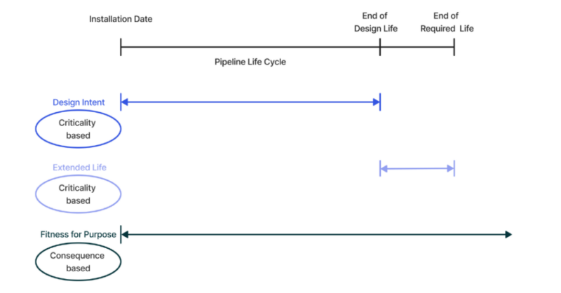
Inspection Strategies based on the Remaining Life of the Pipeline
How Design Intent and Extended Life Strategy Influence the Interval Factor
When the Inspection Strategy is Design Intent or Extended Life, we recommend determining the Interval Factor based on the Criticality and Confidence Rating. A higher Confidence Rating leads to a longer Interval Factor. The Confidence Rating can range from very low to very high and reflects uncertainties in:
- Stability/predictability of the degradation rate,
- Number and quality of previous inspections, and
- Process stability.
The Confidence Rating is assessed for the entire Pipeline. And directly influences the Interval Factor, as it is a function of Criticality and Confidence Rating:
IF = f(Confidence Rating, Criticality)
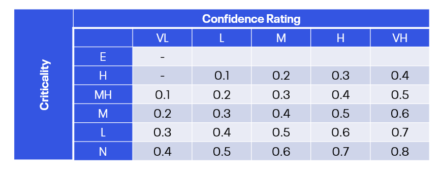
Interval factor calculation table
Criticality itself is measuring both the likelihood of failure (Susceptibility to Failure) and its potential impact i.e. Consequence:
Criticality = f(StF, Consequence)
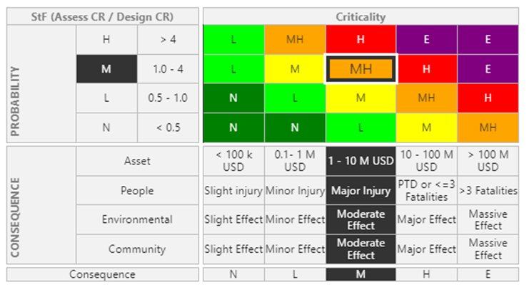
Risk Assessment Matrix
The Susceptibility to Failure (StF) is determined by calculating the ratio of the Assessed Corrosion Rate to the Design Corrosion Rate.
StF = Design Corrosion Rate/Assessed Corrosion Rate
This ratio provides insight into how your actual performance compares to design expectations. If the ratio exceeds 4, it indicates a High StF, while a ratio below 0.5 suggests a negligible StF, as detailed in the table below.

Susceptibility to Failure calculation table
Example:
Let’s dive into a practical scenario. Imagine we have a High Confidence Rating paired with a Medium Consequence of Failure. The design corrosion rate stands at 0.021 mm/year, while our assessed corrosion rate is a more favorable 0.012 mm/year.
Now, let’s calculate the Susceptibility to Failure (StF):
StF = 0.021/0.012 = 1.75
This means that the StF Class is Medium.
Next up is the Criticality assessment. Referring to our Risk-Based Matrix, it’s evident that we’re looking at a Medium-High (MH) classification. Finally, we turn our attention to the Interval Factor. Consulting the Interval Factor table, we see that with a High Confidence Rating and Medium-high Criticality, the Interval Factor is clearly set at 0.4.
Fit for Purpose Inspection Strategy Influences the Interval Factor
When the Inspection Strategy is Fit for Purpose, we recommend determining the Interval Factor based on the Consequence of Failure and Confidence Rating, without considering Criticality. In this case, the Consequence can be specified per section of the pipeline.
IF = f(Confidence rating, Consequence)
Putting it All Together
Now we can finally calculate our Next Inspection Date by using the formula:
Next Inspection Date = Last Inspection Date + (Remaining Life in Years × Interval Factor)
Let’s plug in some numbers. Remember, our last Inspection was on January 1, 2016, with a Remaining Life of 13 years and an interval factor of 0.4. Here’s how it breaks down:
Example:
Next Inspection Date = January 1, 2016 + (13 × 0.4)
That gives us:
Next Inspection Date = January 1, 2016 + 5.2 years
And when we add that up, we land on March 15, 2021.
There you have it! A clear calculation that keeps your pipeline integrity on track.
Risk-Based Pipeline Inspection Planning with Cenosco’s IMS PLSS
External corrosion isn’t just a pipeline problem—it’s a data challenge that demands precise calculations. You can consolidate fragmented data into a cohesive corrosion management strategy by harnessing the power of IMS PLSS (Integrity Management Systems Pipeline and Subsea Systems). The dedicated Risk-Based Assessment module within IMS PLSS enables you to accurately determine the Remaining Life of your Pipeline and schedule future Inspections, ultimately enhancing your Pipeline Inspection Strategy and overall external corrosion management. Ultimately, integrating risk-based assessments into Pipeline Management practices will lead to safer operations, reduced costs, and improved asset performance over time. Our tool doesn’t just allow you to manage external corrosion—it helps you outsmart it.
Want to see what IMS PLSS can do? Request a demo!
Want to learn more about IMS?
Request a demo below to get a first-hand look at its capabilities!

Denis Tkalec Technical writer
Denis Tkalec is a technical writer at Cenosco, specializing in asset integrity management software since 2022. With a background in education and six years in marketing, she turns complex topics into clear, user-friendly content. Inspired by Camus’s belief that “a writer keeps civilization from destroying itself,” she brings precision and care to every manual.