A Crash Course in Fitness for Service (FFS) Assessment for Corroded Pipelines

Fitness for Service (FFS) is not just a technical term; it’s a lifeline for the industrial world, particularly in sectors where aging infrastructure poses significant risks. Imagine a bustling oil rig or a sprawling pipeline system where every inch of metal and weld is constantly scrutinized. These assets are the veins of our economy, and ensuring their integrity is crucial for safety and efficiency. In this blog post, we will embark on a journey to understand the essence of FFS assessments, focusing particularly on pipelines that exhibit defects that result in material loss. 

At its core, Fitness for Service is a quantitative engineering method designed to evaluate the condition of in-service industrial assets—think pipelines, pressure vessels, and storage tanks. The goal? To determine if these critical components can continue to perform their intended functions safely and effectively. The process involves meticulously assessing several factors: design specifications, material properties, operating conditions, and any existing flaws or damage. This comprehensive analysis adheres to established industry standards such as API 579-1/ASME FFS-1, BS 7910, DNV RP-F101, and ASME B31G, which outline methodologies for evaluating component fitness throughout their lifecycle. 

The advantages of conducting FFS assessments are manifold: 

Informed Decision-Making: A structured framework for evaluating asset conditions enables better decisions regarding repairs or continued operation.  

The API 579-1/ASME FFS-1 standard outlines three levels of assessment: 

The primary aim of Fitness for Service assessments is straightforward yet vital: to evaluate whether a component with existing defects is still fit for continued service. For pipelines, this means ensuring that the Safe Working Pressure (P_SW) exceeds the Maximum Allowable Operating Pressure (MAOP). It also answers the question of how long it will remain fit for service. The evaluation also includes calculating corrosion tolerance and determining how much corrosion can occur without compromising structural integrity. This evaluation not only safeguards operations but also helps predict how much life remains in a pipeline. With that information and the help of Risk-Based Assessment, we can calculate the date of the next inspection. 

Safe Working Pressure (P_SW) is a metric that defines the maximum pressure a pipeline can safely handle during normal operations. P_SW must always exceed the Maximum Allowable Operating Pressure (MAOP), representing the highest pressure at which a pipeline can operate without risking failure or damage.   

Now, let’s dive deeper into the mechanics. Picture the internal forces at play when fluids surge through the pipeline. This is where hoop stress comes into play—a silent guardian, wrapping around the pipe and counteracting its natural tendency to burst under pressure. 

Engineers study hoop stress to gauge how much internal pressure a pipe can withstand. It’s like assessing the strength of a bridge before allowing heavy traffic to cross. The formula behind this assessment is Barlow’s Equation, which helps engineers calculate hoop stress based on internal pressure, pipe diameter, and wall thickness. 

σh​=P(D−t)​/2t

Where: 

From hoop stress flows another critical concept: design pressure. This parameter represents the maximum pressure that a pipeline can safely handle, incorporating necessary safety margins. Engineers consider factors like wall thickness and material strength to ensure that pipelines are designed to endure pressures well above what they will face in real-world conditions. It is proactive engineering at its finest—preventing potential failures before they occur. 

To truly grasp how pipelines behave under stress, we must explore their material properties and potential failure mechanisms. Here, the stress-strain curve illustrates how materials respond to applied forces. 

Failure typically occurs between these thresholds, marking a transition from elastic behavior—where materials can spring back—to plastic deformation, where permanent changes take place. 

In practical terms, pipeline failure occurs when hoop stress reaches a critical threshold called flow stress (σflow​). This point signifies that the pipeline can no longer maintain its structural integrity under pressure. Engineers analyze these conditions to establish baseline expectations for material performance under ideal circumstances. 

When corrosion enters the picture, things get trickier. Engineers must assess any defects that could compromise structural integrity. 

For example, if our pipeline has a defect characterized by a certain length (L) and depth (d), we can calculate the area of the defect as: 

A₀ = L x t 

Where: 

To determine the failure pressure of the corroded pipe, we start with the failure pressure of an undamaged pipe and apply a factor known as the Remaining Strength Factor (RSF), which accounts for the impact of corrosion: 

RSF = (1 – A / A₀) / 1 – (A / A₀ x 1 / M) 

Where: 

The failure pressure (P_failure) of a corroded pipeline can then be expressed as the Failure pressure of undamaged pipe times Remaining Strength Factor (RSF) due to corrosion: 

P_failure = 2tσ_flow / (D – t) x RSF 

Or 

P_failure = 2tσ_flow / (D – t) x ((1 – A / A₀) / 1 – (A / A₀ x 1 / M)) 

This equation serves as a universal method for calculating safe working pressures across various pipeline and FFS assessment codes.  

Where: 

By evaluating corrosion extent and its impact on pressure tolerance, they determine how much pressure a corroded pipe can safely handle—ensuring accurate evaluations even in less-than-ideal conditions. 

The Safe Working Pressure (P_SW) emerges from these assessments as an essential guideline for operational limits. It can be calculated using the following formula:  

P_SW = f x 2tσ_flow / (D – t) x RSF 

or 

P_SW = f x 2tσ_flow / (D – t) x ((1 – A / A₀) / 1 – (A / A₀ x 1 / M)) 

Where: 

f = Design factor or safety factor, which accounts for uncertainties in material properties and operating conditions. 

Once we have established safe working pressure, we calculate an Estimated Repair Factor (ERF) based on inspection findings. ERF is defined as: 

ERF = MAOP x P_SW 

This factor helps determine whether corrective actions are necessary: 

For instance, if an inspection reveals an ERF of 0.8 at one point in time but later assessments show an increase beyond 1, it highlights the need for prompt intervention to ensure safety.  

To assess the pipeline’s Fitness for Service, we must evaluate the defects to determine the corrosion tolerance. With this we can then calculate the pipe’s remaining life and next inspection date. Two primary methods dominate this field: ASME B31G and DNV RP-F101. 

ASME B31G was the first to tackle the challenge of calculating safe working pressure in the presence of defects. It includes the original standard, which defines flow stress as 1.1 times the specified minimum yield strength (SMYS), and a modified version that refines this to SMYS plus an additional 69 MPa (about 10 KSI) for greater accuracy. 

On the other hand, DNV RP-F101, introduced in 2010, focuses on ultimate tensile strength (UTS), predicting failure at 0.9 times UTS. This standard simplifies defect shapes, treating them as rectangular, while ASME B31G originally approximated defects as parabolic but later allowed for arbitrary shapes. 

Another critical aspect is the bulging factor, which measures how defects deform under pressure. Smaller defects diminish its significance, while larger ones amplify it.  

To visualize safe working pressures, both standards use the Failure Assessment Diagram (FAD), which translates the Safe Working Pressure equation (P_SW = f x 2tσ_flow / (D – t) x ((1 – A / A₀) / 1 – (A / A₀ x 1 / M))) into a graphical format plotting defect length against depth. Points below the curve indicate safe conditions, while those above signal potential failure risks.

When evaluating defects from In-Line Inspection (ILI) reports, it’s essential to consider maximum allowable depths—80% of Wall Thickness (WT) for ASME and 85% for DNV. Exceeding these thresholds renders defects unsafe. 

In the world of pipelines, defects rarely stand alone. They often cluster together, creating a complex web of potential weaknesses. ASME B31G assesses the defects individually but acknowledges that closely spaced defects can interact as a single larger defect if they are within three times the nominal wall thickness (3t). This interaction can significantly compromise structural integrity. 

In contrast, DNV RP-F101 evaluates each defect individually and considers combinations of adjacent interacting defects. Defects are deemed to interact if their axial distance is less than a specific threshold based on pipe diameter and wall thickness. This criterion helps identify which defects may influence each other. 

The DNV RP-F101 method involves a structured three-step process: 

In the 2010 version of DNV RP-F101, overlapping defects were treated as a single defect with a combined length from the start of the first defect to the end of the last defect in the cluster, using the depth of the deepest defect within that cluster. However, in the 2015 update, overlapping defects are not boxed into one single defect; instead, their individual contributions are considered separately when calculating safe working pressure. 

As we delve deeper into pipeline integrity assessments, we encounter the concept of corrosion tolerance—the maximum allowable corrosion that a pipeline can sustain while still being deemed fit for service. This concept is intertwined with the limit state, defining when a pipeline becomes unsafe to operate. 

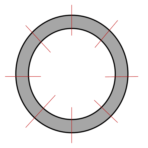
When a pipeline is free of defects, operators must anticipate potential corrosion types—be it general corrosion, grooving, or pitting. For instance, if pitting corrosion is expected, engineers might estimate potential defect lengths as 20 times the depth of the corrosion. This relationship allows them to plot a line on the Failure Assessment diagram from the origin (0,0) based on this length-to-depth ratio. The intersection of this line with safety curve reveals the Corrosion Tolerance (CT) and Minimum Allowable Thickness (MAT) —on the next image the CT and MAT are indicated for grooving corrosion. 

In contrast, if general corrosion is assumed, its length might be represented as 1,000 times the Wall Thickness (WT). This method typically yields lower corrosion tolerance since pitting can lead to deeper material loss than general corrosion. Therefore, accurately identifying the expected type of corrosion is crucial for determining appropriate tolerances.  

When defects are present, the assessment becomes more nuanced. Operators can draw lines on the Failure Assessment Diagram from (0,0) through each defect to ascertain their respective tolerances. The distance between where these lines intersect with the safety curve and where the defect meets the x-axis indicates the Corrosion Tolerances (CT) at the time of the In-Line Inspection (ILI) run.  

Corrosion Tolerance (CT) is calculated for every defect. With ASME B31G, this assessment is straightforward; each defect undergoes a single calculation. However, DNV RP-F101 complicates matters with its iterative process—defects may be assessed multiple times if they interact. This complexity becomes particularly evident when dealing with large datasets. 

When two defects are close enough to interact, they share a common Corrosion Tolerance (CT) due to their combined effects on pipeline integrity. This interaction must be carefully assessed to ensure that Safe Working Pressure (P_sw) calculations remain valid and that the pipeline continues to operate safely. 

As mentioned at the beginning of this article, a Fitness for Service assessment not only determines whether a pipeline is suitable for operation but also estimates how long it can continue to function safely. Once we calculate our Corrosion Tolerance (CT) with the help of the Failure Assessment Curve, we can then estimate the remaining life of the pipeline and calculate when to inspect the pipeline again. 

Remaining Life = CT / CR = 2 mm / 0.1 mm year = 20 years 

This means that under current conditions, the pipeline can operate safely for an additional 20 years before reaching its corrosion limit. 

Next Inspection Interval = Remaining Life × IF 

Using our previous example, if we assume an internal factor of 0.3, the calculation would be: 

Next Inspection Interval = 20 years × 0.3 = 6 years 

This indicates that the pipeline should be inspected again in 6 years to ensure it remains fit for service. 

In pipeline management, Fitness for Service (FFS) assessments are essential for ensuring the safety and continued operation of aging infrastructure. These evaluations not only determine if a pipeline can remain in service but also provide insights into its remaining lifespan. 

Data analysis emerges as the heartbeat of this process, helping operators predict performance and schedule inspections based on calculated remaining life. Cenoco’s IMS – Pipeline and Subsea Systems (PLSS) enables operators to assess pipeline fitness, offering insights into the remaining lifespan. Using methodologies like ASME B31G and DNV RP-F101, operators can accurately evaluate defects and calculate corrosion tolerances. Analyzing the relationship between defects, hoop stress, and Safe Working Pressures supports proactive pipeline management. 

PLSS allows users to assess ILI data through the Fitness for Service module, showing the Safe Working Pressure and Estimated Repair Factor for each defect. Its strength lies in calculating Corrosion Tolerance for individual or grouped defects, factoring in material grade, defect size, and depth. The Risk-Based Assessment module calculates the pipeline’s Remaining Life and next inspection date, with the option to schedule and log inspection findings in the Condition History. This system supports Fitness for Service assessments for pipelines, flowlines, and jumpers made from carbon steel and corrosion-resistant alloys. 

PLSS addresses the most common in-service pipeline defects, specifically volumetric corrosion that can lead to plastic collapse. It focuses on essential yet straightforward Level 1 assessments, such as ASME B31G and DNV RP-F101 Part B. This streamlined approach allows operators to prioritize economic considerations. A more detailed evaluation outside of PLSS is recommended for highly critical pipelines or pipelines subject to strict regulations. 

In conclusion, PLSS is highly effective for managing known, controlled conditions involving volumetric corrosion defects under hoop pressure loading.