Ensuring the integrity of heat exchanger tubes is critical and challenging when it comes to maintaining industrial efficiency. Heat exchangers are vital components in various industries, playing a key role in transferring heat between fluids.
However, inspection becomes a BIG and DIRTY job with bundles containing anywhere from 250 to an overwhelming 5000 tubes. Traditionally, due to concerns over tube conditions and the potential for corrosion in heat exchangers, sites often inspect every single tube. This process is not only laborious but also incredibly time-consuming.
Imagine spending 12 hours just cleaning and inspecting a mere 300 tubes! Moreover, certain corrosion inspection techniques like the Internal Rotary Inspection System (IRIS) necessitate substrate materials to be cleaned meticulously for effective results. Often, this means multiple rounds of washing and inspecting to get accurate data.
Enter Extreme Value Analysis (EVA) – a statistical method revolutionizing how we approach this daunting task. By employing EVA for efficient heat exchanger tube wall thickness calculations, we can confidently reduce the number of tubes inspected without compromising safety or performance.
This not only slashes inspection times significantly but also translates into substantial cost savings. Additionally, EVA helps extend the heat exchanger’s useful life by accurately assessing tube conditions. In this blog, we’ll explore how EVA transforms the heat exchanger inspection process, making it smarter, faster, and more efficient.
Applying Extreme Value Analysis (EVA) for Heat Exchanger Wall Thickness Calculations
Extreme Value Analysis (EVA) is a powerful statistical method for predicting the most extreme values in a dataset. In the context of heat exchangers, EVA is particularly useful for calculating the maximum wall loss from a smaller, representative sample of tubes. The process begins with sampling, where wall thickness readings are taken from a representative selection of tubes within the heat exchanger.
Once the data is collected, it is fitted to a statistical distribution, commonly the Gumbel distribution. This fitting process helps understand the behavior of the extreme values within the dataset. Using this distribution, the maximum wall loss is then extrapolated across the entire heat exchanger, providing a comprehensive view of potential degradation.
From here, the heat exchanger tube wall thickness must be calculated over time. By understanding how the wall thickness changes, it becomes possible to predict the heat exchanger’s remaining useful life. This information is crucial for planning inspections and ensuring the optimal performance of the equipment.
Heat exchanger tube wall thickness calculation steps
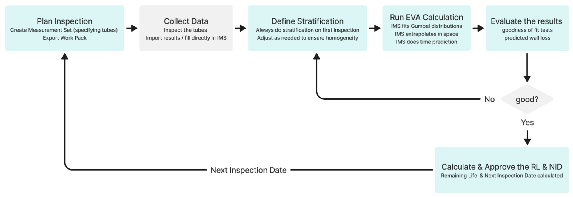
Now that we understand how EVA can be applied to heat exchanger tube wall thickness calculations let’s explore how this process can be practically implemented. We’ll use the workflow from our IMS PEI Software as an example to illustrate this. Here’s a step-by-step breakdown of the process:
- Plan Inspection: Begin by specifying the tubes that need to be measured. Prepare and export the necessary documentation for the inspection.
- Collect Data: Conduct inspections on the selected sample of tubes. This may involve techniques like IRIS, which require the substrate material to be cleaned to a high standard for effective results.
- Define Stratification: Stratification helps manage non-uniform data by creating smaller, consistent groups called strata. Adjusting the stratification as needed ensures the data in each stratum is homogeneous, which is crucial for accurate analysis.
- Run EVA Calculation: The calculation uses the Gumbel distribution to model the extreme values in the collected data. This allows the extrapolation of maximum wall loss across the entire heat exchanger. Traditional corrosion rate models are applied to estimate tube wall thickness over time. (In this case, the EVA calculation is performed using the IMS PEI software.)
- Evaluate the Results: Conduct goodness-of-fit tests to assess the quality of the fitted distribution. If the results are unsatisfactory, return to the stratification step to ensure homogeneous samples. Also, evaluate the predicted wall loss and ensure that the corrosion behavior in the heat exchanger is well understood.
- Calculate and Approve the Remaining Life and Next Inspection Date: Based on the EVA results, calculate the remaining heat exchanger’s useful life and determine the next inspection date. This brings us back to the initial step of planning the next inspection.
The next image visualizes this workflow, providing a clear overview of the entire process.
Ensuring accurate Tube Wall Thickness calculations: Best Practices for Heat Exchanger Inspections
When collecting tube wall thickness data, it’s essential to ensure the sample is both high-quality and representative. High-quality inspections, like those performed using the Internal Rotary Inspection System (IRIS), are highly recommended as they provide accurate and reliable data. However, even with lower-quality inspections, the results tend to be conservative and can still be used.
The sample should represent the entire heat exchanger and be homogeneous to accurately reflect the equipment’s condition. The image below shows a typical representative sample (left) compared to an unrepresentative sample (right), which lacks sufficient spread.
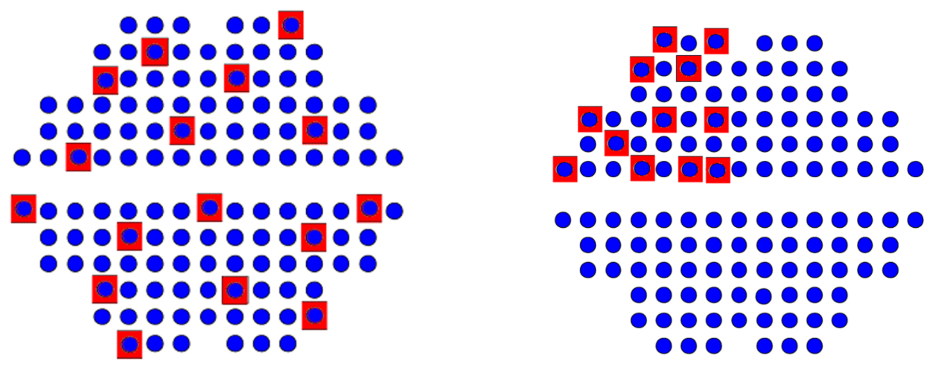
Homogeneous data shows no significant variations or localized areas with higher or lower corrosion rates. When the data is non-homogeneous, stratification is needed. This involves dividing the data into smaller, more uniform groups or strata.
For example, the inlet and outlet sides of the heat exchanger might be separate strata since temperature differences affect corrosion rates. It’s recommended to sample 20-25% of the tubes per stratum, as sampling more could result in overly optimistic estimates. For the first inspection, when establishing a baseline, inspecting up to 100% may be necessary. By following these guidelines, you’ll ensure that your tube wall thickness readings are accurate and reliable.
Assessing the Fit of the Statistical Model: Combining Statistical and Graphical Methods
After fitting the distribution, e.g., Gumbel, to the data, it is essential to assess the goodness of fit using both statistical and graphical methods. Statistical methods include hypothesis tests such as the Kolmogorov-Smirnov test, which evaluates the overall fit quality, and the Anderson-Darling test, which emphasizes the distribution’s tails. These tests provide a quantitative measure of how well the Gumbel distribution represents the data.
In addition to statistical methods, graphical methods should be used to better understand the fit. These include probability plots, exceedance probability plots, and quantile plots.
For example, the quantile plot shown below compares theoretical quantiles to sample quantiles. A quantile divides a dataset into equal-sized intervals (e.g., the median is the 50th quantile, meaning half the data points are below it). If the fit is good, the points in the quantile plot will align along a straight line. The plot includes a line of perfect fit (blue) and confidence bands (green) to highlight deviations.
If most points (red) lie close to the line and within the bands, it indicates the theoretical distribution fits well.
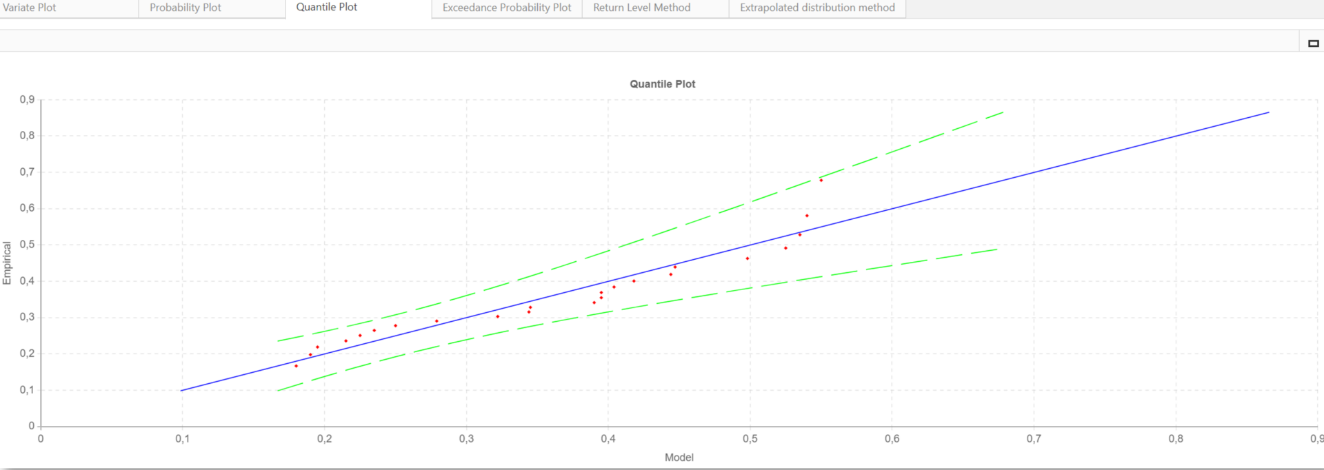
These visual tools help identify discrepancies or patterns that may not be evident through statistical tests alone. It is crucial not to rely solely on statistical methods. Reviewing graphical methods before drawing conclusions ensures a more robust fit evaluation. Furthermore, one should always evaluate the predicted wall loss and ensure that the corrosion behavior is well understood.
Calculating the Tube Wall Thickness for the Entire Heat Exchanger
The aim is to statistically infer the maximum wall loss for the entire heat exchanger. Two methods can be used for this purpose: Return Level and Extrapolated Distribution. These methods help determine the most likely maximum wall loss (extreme value) and its confidence bounds (CBs). Let’s now look at a visual representation to help us understand the distribution of wall loss values and the associated confidence intervals.
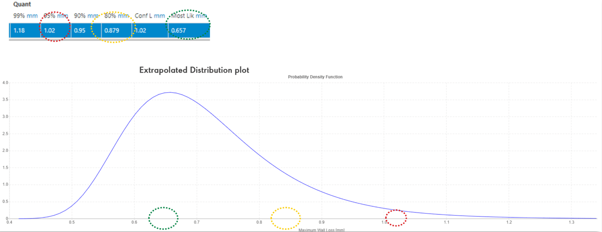
The image above shows an Extrapolated Distribution plot featuring a probability density function curve. The curve peaks at the most likely maximum wall loss value (highlighted by the green circle). It tapers off at both ends, illustrating the distribution of potential maximum wall loss values.
Quantile values, such as the 95th quantile at 1.02mm (marked by the red circle), indicate confidence bounds. This means 95% of the expected maximum wall losses are below 1.02mm, while 80% of the expected maximum wall losses are below 0.879mm (indicated by the yellow circle)
Case Study: Extreme Value Analysis of a Crude Preheater with Three Heat Exchangers
Our case study focuses on inspecting a crude preheater with three trains in operation. These heat exchangers have been running for 25 years, reaching their design life, and the customer wanted to extend their lifespan by at least ten more years. Previously, visual borescope inspections were performed at set intervals to assess tube conditions, but these only provided qualitative data without measuring wall thickness. The customer needed to determine whether replacement was necessary.
One year before the end of life, during a scheduled shutdown, the heat exchangers were inspected using representative samples. This allowed for estimating maximum wall loss and helped decide if it was safe to continue operation for another ten years.
All three heat exchangers had similar results, and we’ll concentrate on one of them. The heat exchanger bundle consists of 120 carbon steel tubes, 23 of which were inspected. Knowledge from previous borescope inspections helped identify the best tubes to examine. The renewal thickness was set at 1.1 mm, with a nominal wall thickness of 2.4 mm.
The inspection took place on October 1, 2023.
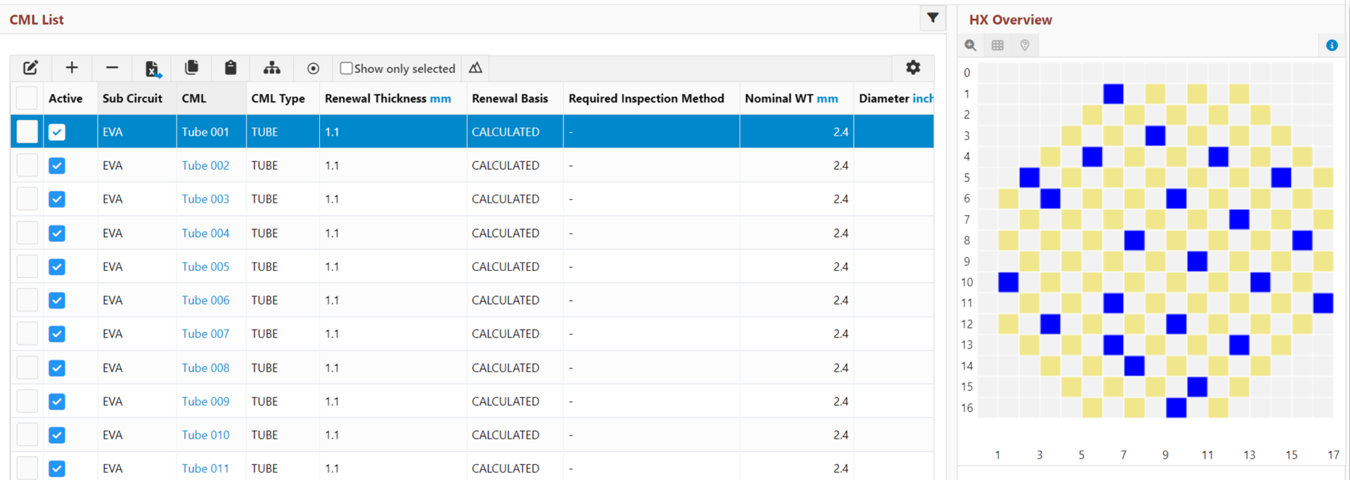
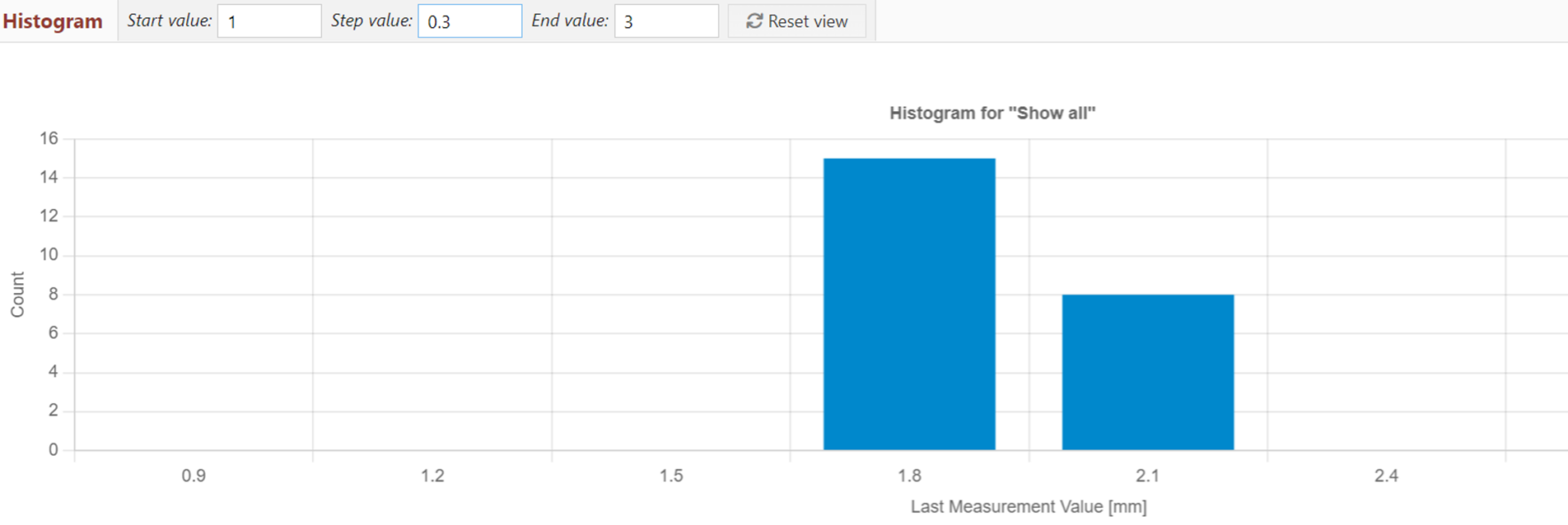
A single homogeneous stratification was sufficient for this heat exchanger. There were no significant variations or localized areas with higher or lower corrosion rates; the values fell within a narrow range, as shown in the histogram below. This confirms that the collected data represented the entire heat exchanger, providing reliable insights into its condition.
Assessing the Fit of the Obtained Statistical Model
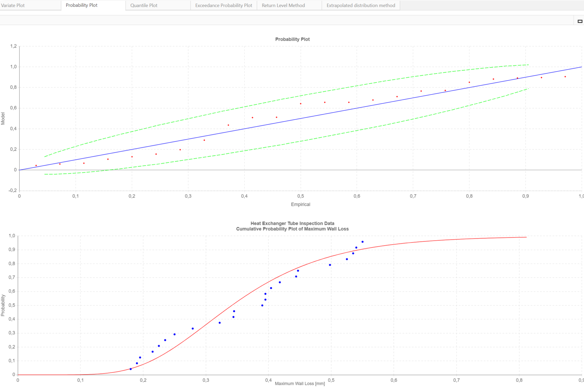
The statistical tests and graphical methods indicated a good fit for the data. Both the Kolmogorov-Smirnov (p-KS) and Anderson-Darling (p-AD) tests showed p-values greater than 0.5, confirming the quality of the fit (see the results below).

The charts also showed that the theoretical distribution aligned well with the sample data, providing confidence in the analysis and confirming a good fit. Below you can see this in the Probability Plots.
Extrapolating the Tube Wall Thickness in Space
Next, the Return Level Method was used to extrapolate the data in space to calculate the maximum wall loss for the entire heat exchanger. The most likely maximum wall loss was 0.816 mm (indicated in red). At the 99% confidence bound, the maximum wall loss was 1.059 mm (indicated in yellow), and at the 80% confidence bound, it was 0.937 mm (indicated in green). The graphs below illustrate these findings.
The upper graph shows the return level curve with the 99% confidence bound, while the lower graph shows the curve with the 80% confidence bound. As you can see, higher confidence bounds lead to more conservative estimates, showing greater wall loss, indicating a thinner remaining tube wall thickness and a shorter useful life for heat exchangers.


Calculating the Heat Exchanger Useful Life and Next Inspection Date
The minimum remaining tube wall thickness and the corrosion rates for the heat exchanger were calculated for various confidence bounds. These calculations enabled the determination of the heat exchanger’s useful life, maximum inspection interval, and next inspection date.
The images below present a detailed breakdown of the results. Firstly, the two tables show the heat exchanger’s minimum remaining wall thickness and corrosion rates at various confidence levels (95%, 90%, and 80%).


The calculation summary then shows the heat exchanger’s useful life (Remnant Life), corrosion rate (Rate), and next inspection date (Next Insp Date) at the 80% confidence level. It’s important to note that the corrosion engineer determines the choice of confidence bound. Typically, using a representative sample and conducting multiple inspections over time increases confidence in the results, allowing for the use of lower confidence bounds.
In this case study, the information gathered from previous borescope inspections gave the engineers enough confidence in the new results to select the 80% confidence bound.

With the heat exchanger’s useful life estimated at 9.5 years (close to the desired ten-year extension), applying the industry-standard half-life concept established the maximum inspection interval (MII) at 4.7 years, with the next inspection scheduled for June 24, 2028. Below is the calculation (at the 80% confidence bound):
Remnant Life = (Minimum Remaining Thickness − Renewal Thickness) / Corrosion Rate=(1.1463mm −1.1mm) / 0.038mm/year = 9.5years
Next Inspection Date = Last Inspection Date + Remnant Life ∗ IF = 1 October 2023+9.5*0.5 = 24 June 2028
These results gave the engineers confidence in the heat exchanger’s condition. Instead of opting for a full replacement, they felt reassured about the necessary actions to keep it operational for another ten years. If the estimated lifespan had been shorter, they might have considered additional options like using corrosion inhibitors to slow down corrosion in the heat exchanger. However, they now knew that no action was required before the next inspection.
Case Study Findings: Reduced Inspection Duration and Turnaround Time
The benefits of using this heat exchanger tube wall thickness calculation approach were significant. By conducting inspections on a representative sample, engineers reduced overall inspection time and preparation activities by at least 40%, streamlining the entire process.
Due to the heat exchangers being part of the critical path, the turnaround time was also shortened by 12%, allowing production to restart sooner than expected. Additionally, a deeper understanding of risks and threats led to an estimated 85% cost savings by avoiding expensive maintenance actions like repairs and replacements. These advantages highlight how EVA makes the heat exchanger inspection process smarter, faster, and more efficient.
Conclusion: EVA ensures efficient and confident inspections
In summary, EVA provides significant time and cost savings for inspections and tube cleaning while ensuring they are performed at the right intervals. By using a representative sample and conducting multiple inspections over time, the conservatism in models can be minimized.
This makes EVA a reliable framework for efficient heat exchanger inspections. For added assurance, IMS PEI allows for independent assessment of tube degradation risks, which can be combined with EVA to determine the optimal time for the next inspection.
Please fill out the form below to see EVA and IMS PEI in action.
Want to learn more about IMS?
Request a demo below to get a first-hand look at its capabilities!

Elsa Tolsma-de Klerk Technical Writer
Elsa is an engineer with a passion for sharing knowledge. She holds a Master’s in Electronic Engineering and spent over a decade at Sasol as an Advanced Process Control Engineer, where she gained hands-on experience in optimization, control systems, and writing technical documentation. Since 2019, she’s been a Technical Writer at Cenosco, now leading the IMS knowledge base and training Academy team.
